Easy Guide: How to Freeze a Row in Excel for Data Stability
Harness the power of Excel to maximize data analysis and management with a useful tool: freezing panes! By learning how to freeze rows or columns in your spreadsheets, you can manage your dataset more efficiently while keeping visibility of crucial information. This guide will cover everything from mastering the Freeze Panes feature in Excel, including instructions for freezing both individual rows and entire columns, unlocking increased productivity that will help streamline all your projects.
Key Takeaways
- Learn how to freeze rows and columns in Excel for improved data stability.
- Explore alternative methods such as splitting panes, creating tables, and printing header rows on every page.
- Troubleshoot common issues with Freeze Panes feature including disabled button or frozen cells not working as expected.
Freezing Rows in Excel: A Step-by-Step Guide
Frustrated by the need to scroll up and down constantly in Excel while working with a large dataset? Freezing rows is an effective way of keeping certain rows static, so you can have them visible as you maneuver around your worksheet. This guide will explain how to lock specific or multiple rows at the top row for more efficient data management on Excel.
To freeze selected (or all) header/data entries from scrolling away when navigating through long datasets: go over each step carefully – select Freeze Rows option under View tab, highlight one or multiple designated lines before selecting it again, click OK if an extra dialogue box appears-and voilà! Those chosen rows won’t budge no matter which direction you choose to look into while on your worksheet.
Freezing the Top Row
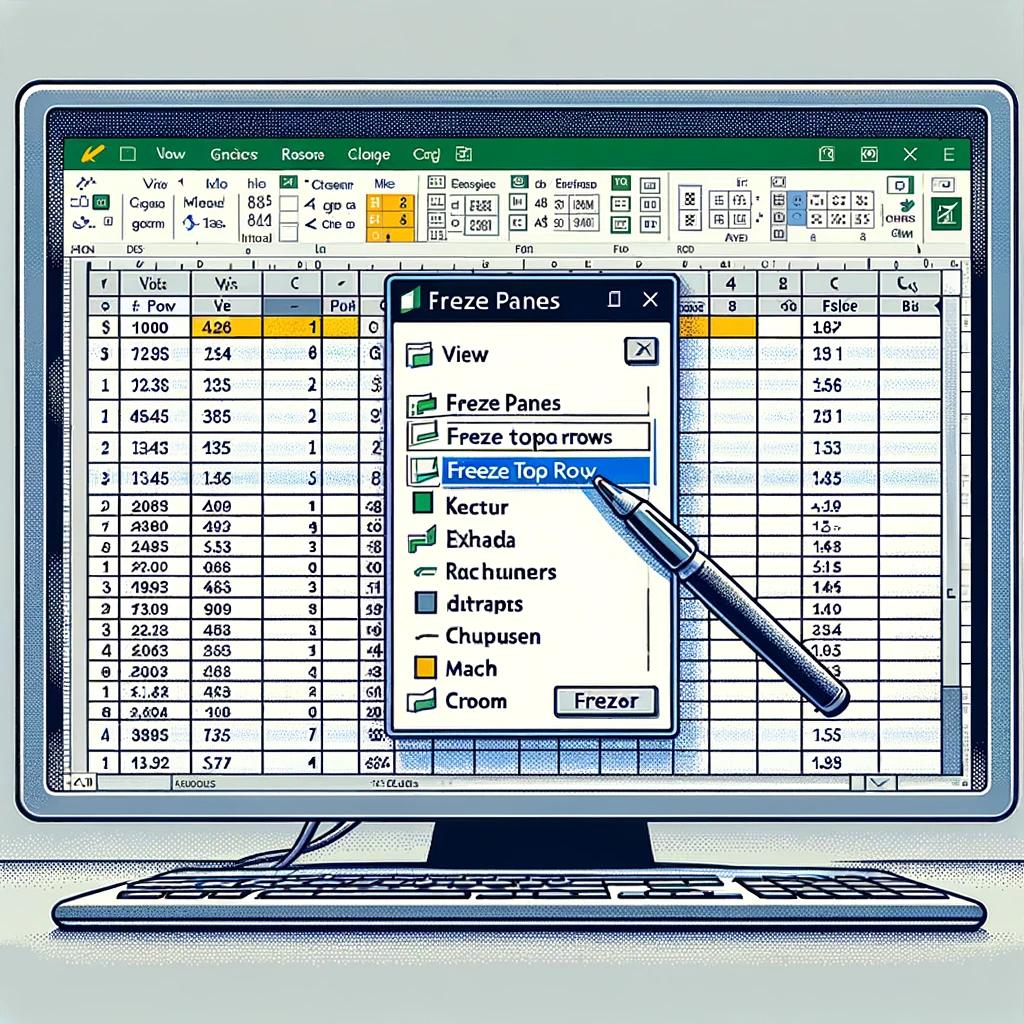
The worksheet’s top row can be frozen to keep it visible while scrolling. To do this, select the row and click on Freeze Panes in the View tab. A grey line appears below your selected cell, which shows that freezing has occurred. Scrolling down now allows you to analyze data more easily without constantly having to return back up each time. If at any point you want unfreeze panes again, just go back into the view tab and choose Unfreeze Panes – then watch as your previously locked-in place top row will disappear!
Freezing Multiple Rows
When navigating through larger datasets, freezing multiple rows can be very helpful. This is especially useful when there are important subheadings or header rows present in the data set. To freeze additional top rows you should start by selecting the row below your desired final one to stay stationary and then click on ‘Freeze Panes’ under the View tab – this will ensure that all of those previously selected upper level items remain visible as you scroll throughout your dataset without having to fixate on a particular position. So don’t forget about this valuable feature if it could help make things simpler for yourself!
Mastering Columns: How to Freeze and Unlock
Knowing how to freeze and lock both columns and rows in Excel is extremely important when you have a wide dataset that needs to be seen even after scrolling. This article will show you the process of freezing individual or multiple columns, including column one, while keeping key data visible at all times on your worksheet.Rows can also easily be frozen so as not to lose track of crucial information whilst viewing your excel document horizontally. Mastering this technique helps maintain visibility across various columns in Excel with just a few steps!
Locking the First Column

If you need to lock the leftmost column of a dataset, simply head over to the View tab and select ‘Freeze Panes’. Then choose ‘Freeze First Column’. The first column will be frozen when there is a grey line appearing on its right side. To unfreeze this same row or any other rows that may have been locked in the process, return to Freeze Panes option under view tab and pick Unfreeze Panes instead, all selected panes will then go back into their normal state again without being secured anymore.
Freezing Multiple Columns
To ensure key data remains visible when scrolling through large datasets, you can easily lock multiple columns in place. Here are the steps to freeze panes for more than one column. Select the cell below your desired last row and select the right-most cell of your required final column from View tab under ‘Window’ group. Then choose ‘Freeze Panes’ option which will make sure that specified rows or columns remain locked while working on the worksheet. This helps quickly manage complex amounts of information with ease by keeping important details always available without needing to scroll back up again every time. Cells outside this area continue functioning normally so users don’t have any hindrance using other functionalities like formulas, etc..
Combining Frozen Rows and Columns

When working with large datasets, freezing both rows and columns, including specific ones, can be quite useful. This ensures that the data is kept visible while scrolling throughout the worksheet. To do this in Excel, go to the ‘View’ tab on its ribbon and select ‘Freeze Panes’. All of the cells around your selection will become frozen. Enabling you to easily work through different parts of your data management efficiently!
Unfreezing Panes: Releasing Locked Rows and Columns
If you need to make changes or return to the original view, unfreezing panes is a quick and easy way to unlock frozen rows and columns. This allows unrestricted scrolling throughout your spreadsheet. To prevent this issue in future editing sessions, using “freeze panes” lets certain selected rows and columns stay put while navigating through it.
To do so: go into View tab > Freeze Panes > Unfreeze Panes - that will remove any locks on designated areas of the worksheet bringing it back as when first opened up for work with zero restrictions from before freezing those same sections of data at some point previously (lock). Remember that if needed once again you can always re-freeze such elements allowing free movement around all other areas except these ones fixed by specific preference simply selecting freeze now instead of un-lock which was just used here!
Troubleshooting Common Issues with Freeze Panes

Have trouble with Freeze Panes in Excel? If the button is disabled or your frozen cells aren’t doing what they should be, understanding common issues and their solutions can help you get back to working smoothly on data management. Learn more about how to resolve complications regarding the freeze feature for both panes and individual cells.
Disabled Freeze Panes Button
The Freeze Panes button can sometimes be unresponsive or unavailable. If this occurs, it could be due to the worksheet being set in Page Layout view or if the workbook is protected. To fix this issue, go to View tab and choose Freeze Panes option before selecting whether you want a top row frozen or just one column from the left side of your sheet locked.Otherwise, there may still be other potential reasons such as cell editing mode enabled within Excel file having corruption issues itself which cause disabling freeze panes for good on that particular version of software program used by user.
Frozen Cells Not Working as Expected
If your frozen cells are not performing as expected, a few underlying issues might be the cause. As a first step in troubleshooting, make sure that you have selected the appropriate active cell before freezing panes and check to see if you’re working on page layout view. It can interfere with this functionality. Verify whether or not Protect Worksheet is enabled, deactivate it for normal functioning of frozen components. If these measures do not fix the issue, try switching from Page Layout Preview back to Normal Preview within View tab settings which may solve any trouble connected with non-working frozen cells/panes.
Alternative Methods for Managing Rows and Columns in Excel

The Freeze Panes feature is a useful way to handle rows and columns in Excel, but there are other approaches you can use such as splitting panes, constructing tables, or printing header rows for every page. Knowing these substitute techniques will provide even more possibilities when managing data with the helpful tool of excel. Thus providing many more options than just freezing your panes.
Splitting Panes for Separate Scrolling

Excel provides an effective way to manage and view your data through splitting panes. This involves creating separate windows of the same spreadsheet, dividing it into distinct parts with their own scroll bars to enable analysis from different sections concurrently.To create split panes in Excel, first you need to select a row column or cell where you want the division located then head over to View tab on ribbon followed by pressing Split button in Windows group. If needed, this can also be removed just double click the split bar and drag up the left side sheet according to requirement.
Creating Tables for Row Locking

Creating tables in Excel to secure rows can be very beneficial for data organization, accuracy and analysis. To get started with this process, select a cell within your dataset then go to the Home tab where you will find an option labeled ‘Format as Table’ which gives you access to pick from various table styles that fit best your requirements. Row locking through tables offers enhanced visibility over datasets alongside prevention of any accidental changes while also making it easier for comparing different pieces of information. Although convenient, users should bear in mind certain limitations such as being unable to expand pre-existing protected sheets or add additional rows on other ones already locked down by protection settings.
Printing Header Rows on Every Page
When printing out a large volume of data in Excel, it’s vital to incorporate header rows on each page for consistency and easy analysis. To do this, go to the “Page Layout” tab, click “Print Titles” located within the group labeled “Page Setup”, then select the row containing your desired headers you want repeated throughout every printed page.Having these headings shown consistently across all pages makes it easier for understanding and working with information that could span multiple documents. This way columns or labels will always be clearly visible, providing better insight into underlying datasets.
Summary
Gaining knowledge of Excel’s Freeze Panes capability can improve data management and enhance output. This guide has prepared you to be able to freeze/unfreeze rows and columns, tackle issues that may arise when doing so, as well as investigating other methods for handling said rows and columns in the program itself. Thus providing visibility into essential details at all times. With these tools on hand now, taking charge of any large set of records is feasible, preserving indispensable information along with it!
Frequently Asked Questions
How do you freeze specific rows in Excel?
To ensure specific rows are frozen in Excel, click the View tab and select Freeze Panes > Freeze Panes. The row you chose to freeze should then remain indicated by a grey line beneath it, with all other panes staying frosty as well.
What is the shortcut key to freeze rows in Excel?
The Excel shortcut to freeze rows is ‘ALT+W+F+R’, which will lock the top row in place. On the other hand, use of ‘ALT+W + F + C’ can be made for freezing a single column (leftmost). It’s quite simple and efficient to keep various rows or columns intact with these combinations while using Excel as they help preserve information without sacrificing any fact.
How do I freeze rows in sheets?
To lock in place certain rows, go to View on Google Sheets and hover over or click the Freeze choice. Pick either a specific number of rows or columns that you would like to freeze.
Why won't my top row freeze in Excel?
If you’re having difficulty freezing the top row of your Excel sheet, it may be because you have opened your workbook in Page Layout view. This display doesn’t allow for freeze panes to be enabled. To resolve this issue, simply switch over to the Page Break Preview tab on View and then the frozen option can now become available. Freeze pane is an important feature which keeps a specific row or column visible no matter how far down/across one scrolls within their spreadsheet document. Thus allowing for the future.
How can I unfreeze panes in Excel?
From the View tab, select Unfreeze Panes from the Freeze Panes command dropdown menu to unfreeze panes in Excel. This is done by freezing and then thawing previously-frozen sections of cells or sheets within your spreadsheet program.